Chapter 1 R and RStudio
The purpose of this section is to get you started learning a new language and learning how to program! Throughout BIOSCI220 you will be introduced to tools required to critically analyse and interpret biological data.

Learning objectives
-
Define the difference between
RandRStudio - Express the benefits and issues associated with these software being used in the scientific community. Specifically,
- summarise the benefits and drawbacks associated with the open-source paradigm,
- discuss the concept of reproducible research and outline its importance
- Distinguish between different data types (e.g., integers, characters, logical, numerical)
-
Explain what an
Rfunction is; describe what an argument to anRfunction is -
Explain what an
Rpackage is; distinguish between the functionsinstall.packages()andlibrary() -
Explain what a working directory is in the context of
R -
Interpret and fix basic
Rerrors such as
## Error in library(fiddler): there is no package called 'fiddler'and
## Error in file(file, "rt"): cannot open the connectionR function to read in a .csv data; carry out basic exploratory data analysis using tidyverse (e.g., use the pipe operator, %>% when summarizing a data.frame)
1.1 What are R and RStudio?
R is a language, specifically, a programming language. Think of it as the way you can speak to your computer to ask it to carry out certain computations. RStudio is an integrated development environment (IDE). This means it is basically an interface, albeit a fancy one, that makes it easier to communicate with your computer in the language R. The main benefit is the additional features it has that enable you to more efficiently speak R.
You can think of R as the engine to RStudio’s dashboard.

Note R and RStudio are two different pieces of software; for this course you are expected to download both. As you’d expect, the dashboard depends on the engine (i.e., RStudio depends on R) so you have to download R to use RStudio!
1.1.1 Why are you learning to program?
The selling pitch of this course states that …biological research has actually been heavily quantitative for 100+ years… and promises that …it is now essential for biology students to acquire skills in working with and visualizing data, learning from data using models…. We’re not making it up!
If you need convincing that quantitative and programming skills are essential to graduate in all scientific disciplines have a read of the following.
Throughout this course we will be programming using R. R is a free open-source statistical programming language created by Ross Ihaka (of Ngati Kahungunu, Rangitane and Ngati Pakeha descent) and Robert Gentleman, here at UoA in the Department of Statistics! It is widely used across many scientific fields for data analysis, visualization, and statistical modeling. Proficiency in R will enable you to wrangle and explore datasets, conduct statistical analyses, and create visualizations to communicate your findings. These are all essential tools required in any scientific discipline.
TASK Go to the Statistics Department display in the science building foyer (building 302) to see a CD-Rom with the first ever version of R.
RStudio is an integrated development environment (IDE) for the R programming language. It serves as a user-friendly workspace, offering additional tools for coding, data visualization, and project management. RStudio simplifies the process of learning R by providing a structured interface with many built-in tools to help organize workflow, fostering a systematic approach to data analysis and research.
TASK Research the meaning of open-source software and briefly outline the pros and cons of this in the context of statistical analysis.
1.2 Installing R and RStudio
NOTE: RStudio depends on R so there is an order you should follow when you download these software!
TASK Follow the instructions below to install R and RStudio. Here are some step-by-step instructional videos you might find useful
Download and install
Rby following these instructions. Make sure you choose the correct operating system; if you are unsure then please ask either a TA or myself.Download and install
RStudioby going here choosing RStudio Desktop Open Source License Free and following instructions. Again if you are unsure then please ask either a TA or myself.Check all is working
- Open up
RStudiofrom your computer menu, the icon will look something like this (DO NOT use this icon
  , this is a link to
 Rand will only open a very basic interface) - Wait a little and you should see
RStudioopen up to something similar to the screenshot below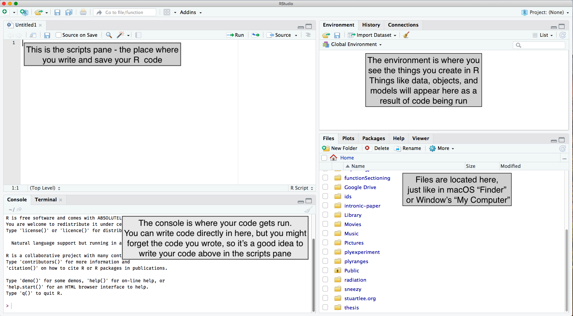
- Pay close attention to the notes in the screenshot and familiarise yourself with the terms.
- Open up
TASK Once you have both R and Rstudio installed, in the Console next to the prompt type 1:10 and press enter on your keyboard. Your computer should say something back you (in the Console)! What do you think you were asking it to do? Does the output make sense?1
1.3 Getting started with R
Open up RStudio from your computer menu, the icon will look something like this ![]() . Identify the following panes
. Identify the following panes
- Console Pane: The console is where you can directly interact with R. You can type and execute R commands line by line, and the results will be displayed in the console pane. It’s an interactive space for immediate feedback and testing.
- Environment/History Pane: This pane provides information about the current
Renvironment, including a list of variables, data frames, and other objects in your workspace. It also shows the history of commands that you have executed in the console. - Files/Plots/Packages/Help Pane: This pane is a multi-purpose pane that can display different tabs depending on your current activity. It can show the file structure of your project, display plots and visualizations, provide information about installed packages, and offer help documentation.
These three panes will likely be the ones to appear by default. There is a fourth pane, one which you will have to open yourself. This is the Code/Source Pane and is where you can write, edit, and save your R script or code files. It’s the primary workspace for creating and modifying your R code.
TASK Read the text at the top of your Console. What does the very first line say? Mine says version 4.3.1 (2023-06-16) -- "Beagle Scouts". Read this blog to find our what this means.
1.3.1 The Code/Source Pane
R Scripts (a .r file)
Go File > New File > R Script to open up a new Script
If you had only three panes showing before, a new (fourth) pane should open up in the top left of RStudio. This file will have a .r extension and is where you can write, edit, and save the R commands you write. It’s a dedicated text editor for your R code (very useful if you want to save your code to run at a later date). The main difference between typing your code into a Script vs Console is that you edit it and save it for later! Remember though the Console is the pane where you communicate with your computer so all code you write will have to be Run here. There are two ways of running a line of code you’ve written in your Script
- Ensure your cursor is on the line of code you want to run, hold down Ctrl and press Enter.
- Ensure your cursor is on the line of code you want to run, then use your mouse to click the Run button (it has a green arrow next to it) on the top right of the Script pane.
TASK Type 1:10 in your Script and practise running this line of code using both methods above. Not that if you’ve Run the code successfully then your computer will speak back to you each time via the Console.
1.3.2 R basics
| Term | Description |
|---|---|
Script |
A file containing a series of R commands and code that can be executed sequentially. |
Source |
To execute the entire content of an R script, often done using the “Source” button in RStudio. |
Running Code |
The process of executing R commands or scripts to perform specific tasks and obtain results. |
Console |
The interactive interface in RStudio where R commands can be entered and executed line by line. |
Commenting |
Adding comments to the code using the # symbol to provide explanations or annotations. Comments are ignored during code execution. |
Assignment Operator |
The symbol <- or = used to assign values to variables in R. |
Variable |
A named storage location for data in R, which can hold different types of values. |
Data Type |
The classification of data into different types, such as numeric, character, logical, etc. |
Object |
A data structure that holds a specific type of data. Objects are used to store and manipulate data, and they can take various forms depending on the type of information being represented. |
Logical Operator |
Symbols like ==, !=, <, >, <=, and >= used for logical comparisons in conditional statements. |
Function |
A block of reusable code that performs a specific task when called (e.g., mean(c(3, 4)). |
Argument |
The input values that are passed to the function when it is called. |
Error Handling |
The process of anticipating, detecting, and handling errors that may occur during code execution. |
Debugging |
The process of identifying and fixing errors or bugs in the code. |
Workspace |
The current working environment in R, which includes loaded data, variables, and functions. |
Commenting
Comments are notes to yourself (future or present) or to someone else and are, typically, written interspersed in your code. Now, the comments you write will typically be in a language your computer doesn’t understand (e.g., English). So that you can write yourself notes in your Script you need to tell your computer using the R language to ignore them. To do this precede any note you write with #, see below. The # is R for ignore anything after this character.
## IGNORE ME
## I'm a comment
## I repeat I'm a comment
## I am not a cat
## OK let's run some code
2 + 2
## [1] 4
## Hmm maybe I should check this
## @kareem_carr ;-)
Now remember when you want to leave your R session you’ll need to Save your Script to use it again. To do this go File > Save As and name your file what you wish (remember too to choose a relevant folder on your computer, or as recommended use the .Rproj set-up as above).
Data types
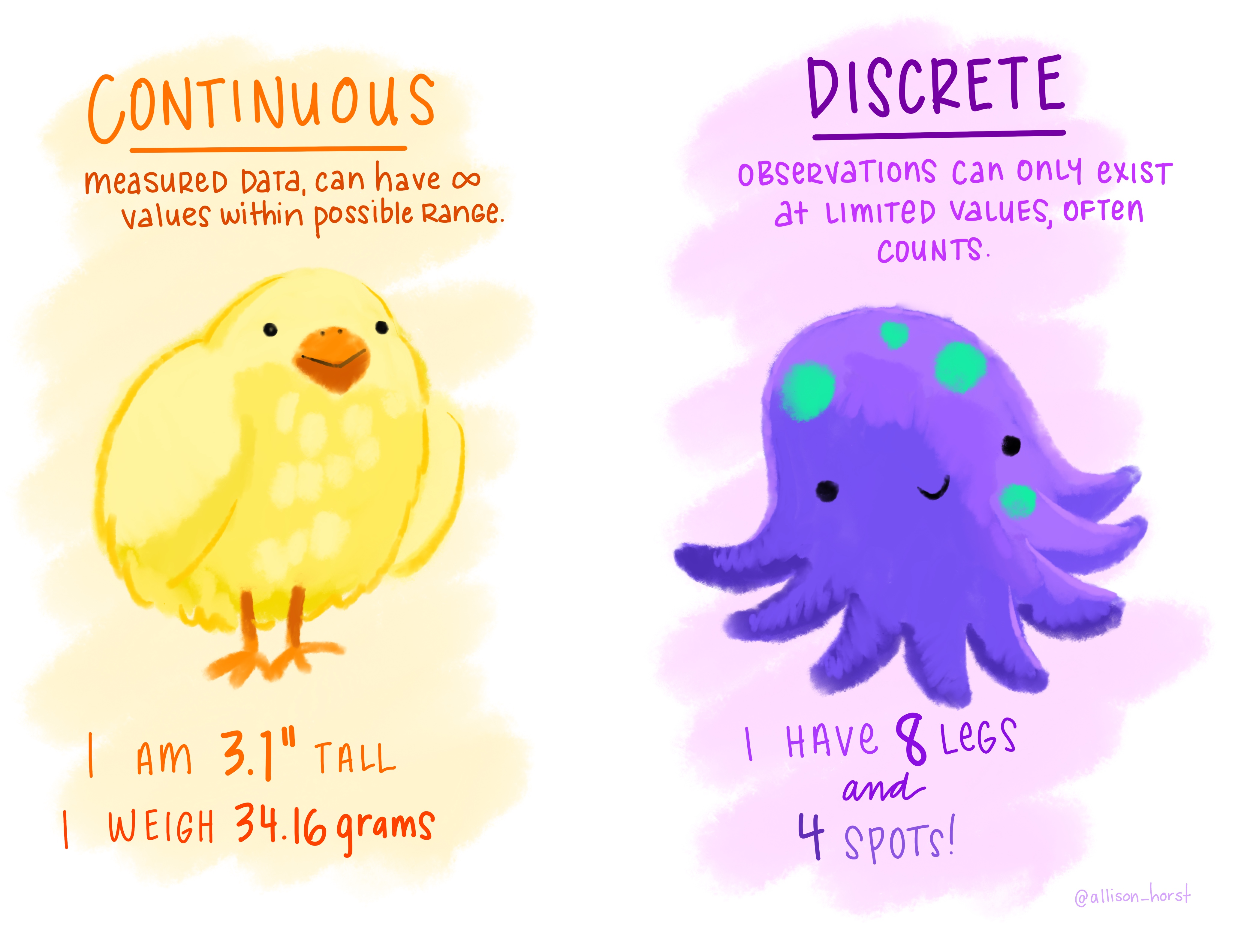
Artwork by @allison_horst
Here we’re covering data types in R (e.g., integers, doubles/numeric, logical, and characters).
- Integers are whole values like 1, 0, 220. These are classified
"integer"orintinR. - Numeric values are a larger set of values containing integers but also fractions and decimal values, for example -56.94 and 1.3. These are classified
"numeric"ornumordblinR. - Logical values are either TRUE or FALSE. These are classified
"logical"orlglinR. - Characters are text such as “Charlotte”, “BIOSCI220”, and “Statistics is the greatest subject ever”. Note that characters are denoted with the quotation marks around them and are classified
"character"orchrinR.
## As an example we're going to ask our computer, using R, what it classified the character string "Charlotte" as
class("Charlotte")
## [1] "character"
Creating Objects
Objects are created (or assigned) values using the symbols <- (an arrow formed out of < and -). Like we, typically, write an equation the left-hand side is the Object we’re defining (creating) and the right-hand side is the stuff we’re defining it as. For example, below I’m creating the Object my_name and assigning it the character string of my first name.
So now the Object my_name ‘contains’ the value "Charlotte". Another assignment to the same object will overwrite the content.
To check the content of an Object you can simply as your computer to print it out for you (in R).
Note: R is case sensitive: it treats my_name and My_Name as different objects.
An object can be assigned a collection of things:
my_names <- c("Charlotte", "Moragh", "Jones-Todd")
my_names
## [1] "Charlotte"  "Moragh"     "Jones-Todd"
some_numbers <- c(1,4,5,13,45,90)
some_numbers
## [1]  1  4  5 13 45 90
An Object can also be an entire dataset (see later in this section)!
R functions
Functions (or commands) perform tasks in R. They take in inputs called arguments and return outputs. Functions often have both mandatory and optional arguments: mandatory arguments must be provided for the function to execute correctly, while optional arguments have default values but can be customized by the user. You can either manually specify a function’s arguments or use the function’s default values. For example, the function seq() in R generates a sequence of numbers. If you just run seq() it will return the value 1. That doesn’t seem very useful! This is because the default arguments are set as seq(from = 1, to = 1). Thus, if you don’t pass in different values for from and to to change this behaviour, your computer just assumes all you want is the number 1. You can change the argument values by updating the values after the = sign. If we try out seq(from = 2, to = 5) we get the result rseq(from = 2, to = 5)` that we might expect.
R packages
An R package is simply a collection of functions! Typically all focused on a particular type of procedure.
The base installation of R comes with many useful packages as standard and these packages will contain many of the functions you will use on a daily basis (e.g., mean(), length()). However, often we wish to do more than base R offer! To do this we need to access all the other amazing packages there are in the Rverse.

The Comprehensive R Archive Network(CRAN) is like a centralised library with thousands of books (packages) in stock.
To access the contents of a book (package) you first need to request it for (install it into) your local library (your computer):
## note that <the.package.name> is just a placeholder
## and should be replaced by your desired package name
install.packages('<the.package.name>')

Note that you ou can only access books in your local library.

To access the knowledge in a particular book (use the function is the package) you need to tell your computer via R to go get the book of the shelf. Then you have access to all the functions it contains!
## note that <the.package.name> is just a placeholder
## and should be replaced by your desired package name
library(<the.package.name>)
Working directories
You need to tell your computer where to look!
Look at the top of your Console. You will see something like ~/Desktop/ or C://Users/… (it won’t be an exact match of course). This is the ‘address’ of where your computer is looking. Now, run getwd() and see what output you get (it will be the same as written on the top of your Console pane. This is because getwd() stands for get the current working directory (i.e., the current directory you are currently working in) e.g.,
You should ensure that you are aware of which directory you’re working in (which folder RStudio is looking in by default) as this is important later on when we come to reading in files and saving our work!
What if you’re not where you want to be (i.e., you are looking in the wrong folder)?
Click Session > Set Working Directory > Choose Directory > Chose where you want to go
Now notice that something has been written in your Console something similar to setwd("~/Git/BIOSCI220/data"). Now setwd() stands for set your workingdirectory. If you know the address of the directory you want to work in without having to point-and-click you could use this command directly, in this case you’ve used the point-and-click to do it and RStudio has helpfully written out your choices as an R command.
Getting help
How do we know what a function does? Let’s say we want to learn more about the function mean() (we can take a wild guess at what it calculates, but… what if we didn’t know for sure. There are two ways we can ask within RStudio
or
The code above will open up the official R documentation (or man pages) for the function mean(). Every function has a corresponding man page that provides comprehensive information on its usage, required arguments, return value, and often gives user examples. You should always consult the documentation to ensure that what you believe you are asking is indeed what you are asking your computer to do.
1.4 Dealing with data
Reading in data from a .csv file
First off download the paua.csv file from this link onto your computer (remember which folder you saved it in!)
This dataset contains the following variables
Ageof P\(\overline{\text{a}}\)ua in years (calculated from counting rings in the cone)Lengthof P\(\overline{\text{a}}\)ua shell in centimetersSpeciesof P\(\overline{\text{a}}\)ua: Haliotis iris (typically found in NZ) and Haliotis australis (less commonly found in NZ)
To read the data into RStudio
In the Environment pane click Import Dataset > From Text (readr) > Browse > Choose your file, remembering which folder you downloaded it to > Another pane should pop up, check the data looks as you might expect > Import
You should now notice that in the Environment pane there is something listed under Data (this is the name of the data.frame Object containing the data we will explore)
Now notice how in the Console a few lines of code have been added. These are the commands you were telling your computer via the point-and-click procedure you went through! Notice the character string inside read_csv()… This is the full ‘address’ of your data (the folder you saved it in). When you tell your computer to look for something you need to tell it exactly where it is! Remember the getwd() command above, this tells you the default location RStudio will look for a file, if your file is not in this folder you have to tell it the full address.
Alternatively we could read this data directly into R using the URL (and the readr package, which is part of the tidyverse collection):
paua <- readr::read_csv("https://raw.githubusercontent.com/STATS-UOA/databunker/master/data/paua.csv")1.4.1 Using functions to look at the data
Automatically RStudio has run the command View() for you. This makes your dataset show itself in the top left pane. It’s like looking at the data in Excel. Follow along with the commands below, I recommend that you open up a new Script and use that to write and save your commands for later. Don’t forget to ensure you have read the paua into your session (all commands below assume that your data Object is called paua, if you’ve called it something different then just replace paua with whatever you’ve called it below.
Now let’s go ahead and use some functions to ask and answer questions about our data. The first thing you should always do is view any data frames you import.
- Let’s have a look at your data in the Console
paua
## # A tibble: 60 × 3
##    Species            Length   Age
##    <chr>               <dbl> <dbl>
##  1 Haliotis iris        1.8   1.50
##  2 Haliotis australis   5.4  11.9
##  3 Haliotis australis   4.8   5.42
##  4 Haliotis iris        5.75  4.50
##  5 Haliotis iris        5.65  5.50
##  6 Haliotis iris        2.8   2.50
##  7 Haliotis australis   5.9   6.49
##  8 Haliotis iris        3.75  5.00
##  9 Haliotis australis   7.2   8.56
## 10 Haliotis iris        4.25  5.50
## # ℹ 50 more rows
So, what does this show us?
A tibble: 60 x 3: Atibbleis a specific kind of data frame inR. Ourpauadataset has60rows (i.e., 60 different observations). Here, each observation corresponds to a P\(\overline{a}\)ua shell.3columns corresponding to 3 variables describing each observation.
Species,Length, andAgeare the different variables of this dataset.- We then have a preview of the first 10 rows of observations corresponding to the first 10 P\(\overline{a}\)uashells. ``
... with 50 more rowsindicates there are 50 more rows to see, but these have not been printed (likely as it would clog our screen)
Let’s look at some other ways of looking at the data.
- Using the
View()command (recall from above) to scroll through the data in a pop-up viewer
- Using the
glimpse()command from thedplyrpackage for an alternative view
library(dplyr)
glimpse(paua)
## Rows: 60
## Columns: 3
## $ Species <chr> "Haliotis iris", "Haliotis australis", "Haliotis australis", "…
## $ Length  <dbl> 1.80, 5.40, 4.80, 5.75, 5.65, 2.80, 5.90, 3.75, 7.20, 4.25, 6.…
## $ Age     <dbl> 1.497884, 11.877010, 5.416991, 4.497799, 5.500789, 2.500972, 6…
glimpse() will give you the first few entries of each variable in a row after the variable name. Note also, that the data type of the variable is given immediately after each variables name inside < >.
TASK! Try running the following operations on the paua data object. What do you think each is asking?
head(paua)tail(paua)paua[1:10,]paua[,2]paua$Age
1.5 Error handling and debugging
Sometimes rather than doing what you expect it to your computer will return an Error message to you via the Console prefaced with Error in… followed by text that will try to explain what went wrong. This, generally, means something has gone wrong, so what do you do?
- Read it! THE MESSAGES ARE WRITTEN IN PLAIN ENGLISH (MOSTLY)
- DO NOT continue running bits of code hoping the issue will go away. IT WILL NOT.
- Try and work out what it means and fix it (some tips below).
Interpreting R errors is an invaluable skill! The error messages are designed to be clear and informative. They aim to tell might be going wrong in the code. These messages typically contain information about the type of error hinting at how you might fix it. For example, if there is a typo in a function or variable name, R will produce an error like "Error: object 'variable_name' not found.” This suggests that R couldn’t find the specified object variable_name.
Understanding error messages involves paying attention to the details, such as the error type (e.g., syntax error, object not found, etc.), and the specific line number where the error occurred! You should always run your code line-by-line, especially if you are new to programming. This means that the execution of each line of code is done in in isolation, providing immediate feedback and pinpointing the exact location where an error occurs. If the meaning or solution to an error isn’t immediately obvious then make use of the documentation (RTFM) and even technology. Online platforms like Stack Overflow or RStudio Community and tools like ChatGPT can often be your friend! It is very unlikely that you are the first one to have encountered the error and some kind soul with have posted a solution online (which the AI bot will have scraped…). However, it’s crucial to approach online answers carefully. You need to first understand the context of your error and use your knowledge about your issue to figure out if the solution is applicable (this gets easier with experience).
It is always best to try debugging yourself before blindly following a stranger’s advice. Debugging is a crucial aspect of R programming and the process itself helps solidify your understanding. There are several widely used methods that help identify and resolve issues in your code, two are outlined below.
- Print debugging involves actively printing out objects and asking the software to display variable values or check the flow of execution. For example, if you get this error message
"Error: object 'variable_name' not found.I might askRto print out what objects do exist in my workspace, it could be that a previous typo means that the objectvariable_namexists. - Rubber duck debugging is a useful debugging strategy where you explain your code or problem out loud (as if explaining it to a rubber duck). Honestly it works! The process helps clarify your thoughts and identify issues even before seeking external help.
The table below summaries some common R issues and errors and their solutions.
| Error/Issue | Description | Solution |
|---|---|---|
| Syntax Error | Incorrect use of R syntax, such as missing or mismatched parentheses, braces, or quotes. |
Carefully review the code, check for missing or mismatched symbols, and ensure proper syntax is used. |
| Object Not Found | Attempting to use a variable or function that hasn’t been defined or loaded into the workspace. | Check for typos in variable or function names, ensure the object is created or loaded, and use correct names. |
| Package Not Installed/Loaded | Trying to use a function from a package that is not installed or loaded into the environment. | Install the required package using install.packages("package_name"), and load it using library(package_name). |
| Undefined Function/Variable | Using a function or variable that hasn’t been defined or is out of scope. | Define the function or variable, or check its scope within the code. |
| Data Type Mismatch | Operating on data of incompatible types, such as performing arithmetic on character data. | Ensure that data types are compatible, and consider using functions like as.numeric() or as.character() for conversions. |
| Misuse of Assignment Operator | Using the wrong assignment operator (= instead of <- or vice versa). |
Be consistent with the assignment operator, and use <- for assignment in most cases. |
| Missing Data | Dealing with missing values in the data, leading to errors in calculations or visualizations. | Handle missing data appropriately, using functions like na.omit() or complete.cases(). |
| Index Out of Bounds | Attempting to access an element in a vector or data frame using an index that is out of range. | Check the length of the vector or data frame and ensure the index is within bounds. |
| Failure to Load a File | Issues with loading a data file using functions like read.csv() or read.table(). |
Check the file path, file format, and encoding. Confirm that the file exists in the specified location. |
| Incorrect Function Arguments | Providing incorrect arguments or parameters to a function, leading to errors. | Refer to the function’s documentation to understand the correct parameters and ensure proper usage. |
Sometimes your computer will return a warning messages to you prefaced “Warning:”. These can sometimes be ignored as they may not affect us. However, READ THE MESSAGE and decide for yourself. Occasionally, also your computer will write you a friendly message, just keeping you up-to date with what it’s doing, again don’t ignore these they might be telling you something useful!
TASK Keep a bug diary! Each time you get an error message, see if you can solve it and keep a diary of your attempts and solution.
You should have seen the numbers 1 to 10 printed out as a sequence.↩︎